
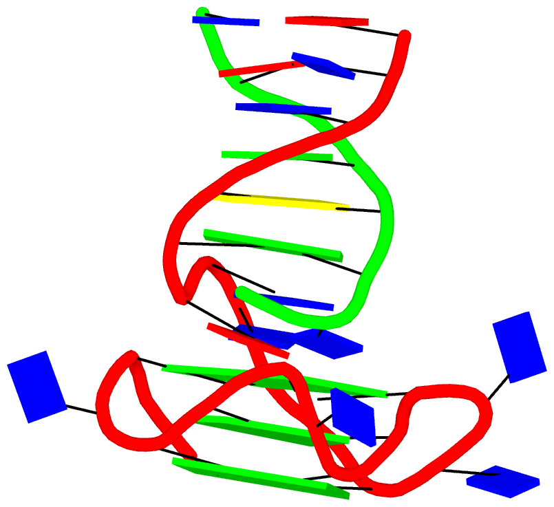
Crystal structure of SARS-CoV-2 stem–loop 5 (SL5) (PDB id: 9E9Q; Jones CP, Ferré-D'Amaré AR. 2025. Crystallographic and cryoEM analyses reveal SARS-CoV-2 SL5 is a mobile T-shaped four-way junction with deep pockets. RNA 31: 949–960). The T-shaped four-way junction of the coronavirus SL5 structural element provides a starting point for examining the structures of larger RNA motifs and their interactions with other molecules. Image highlighting the four arms of the junction. The RNA backbone is depicted by a gray ribbon. The bases within the arms of the junction are colored respectively in blue, red, yellow, and cyan. Cover image provided by X3DNA-DSSR, an NIGMS National Resource for Structural Bioinformatics of Nucleic Acids (R24GM153869; skmatics.x3dna.org). Image generated using DSSR and PyMOL (Lu XJ. 2020. Nucleic Acids Res 48: e74).
As the developer of DSSR, I am thrilled to see its application in cutting-edge research across multiple disciplines. Below is a list of four recent publications that highlight how DSSR has been utilized, underscoring its versatility and significance in structural bioinformatics.
In the Geng et al. (2025) Nucleic Acids Research (NAR) paper, titled 'Revealing hidden protonated conformational states in RNA dynamic ensembles', DSSR is simply cited as follows:
All bp geometries, hydrogen-bond, backbone, stacking, and sugar dihedral angles were calculated using X3DNA-DSSR [77].
In the preprint by Gordan et al. (2025), titled 'High-throughput characterization of transcription factors that modulate UV damage formation and repair at single-nucleotide resolution', DSSR is cited as follows:
Step base stacking, base pair shift, base pair slide, interbase angle, pseudorotation angle, and sugar puckering classifications of nucleobases were computed using X3DNA-DSSR (v2.5.0)75. Base stacking was defined as the overlapping polygon area in Å2 when projecting the dipyrimidine base ring atoms (excluding exocyclic atoms) into the mean base pair plane76. The sugar ring pseudorotation phase angle of each pyrimidine was also calculated using X3DNA-DSSR as described by Altona, C. & Sundaralingam, M.77 Interbase angle was defined as sqrt(propeller2+buckle2) per the X3DNA-DSSR documentation.
Figure 6: TF Binding Induces Structural Distortion Favorable to UV Dimerization is highly informative, particularly panel (a), which illustrates the ensemble of structural parameters that predispose dipyrimidines to cyclobutane pyrimidine dimers (CPD) or 6-4 pyrimidine-pyrimidones (6-4 PP) formation. DSSR is designed as an integrated software tool, offering a comprehensive suite of structural parameters not found in any other single tool I am aware of. Despite this, the innovative use of DSSR by Gordan et al. exceeds my expectations and demonstrates its versatility.
In the preprint by Kubaney et al. (2025) from the Baker group, titled 'RNA sequence design and protein-DNA specificity prediction with NA-MPNN', DSSR is cited as follows:
On the pseudoknot subset, we evaluate additional structure‐ and reactivity‐based metrics. DSSR v2.3.241 is used to extract the ground‐truth secondary structure from the native crystal structures. For each designed sequence, RibonanzaNet predicts 2A3 reactivity profiles, from which we compute predicted OpenKnot scores (see https://github.com/eternagame/OpenKnotScore)31 using the predicted reactivity together with the DSSR ground truth.
In a recent NSMB paper from the Baker group, titled 'Computational design of sequence-specific DNA-binding proteins', 3DNA is cited as follows:
RIF docking of scaffolds onto DNA targets (DBP design step 1) Structures of B-DNA for each target (Supplementary Table 2) were generated by (1) using the DNA portion of PDB 1BC8 (ref. 60), PDB 1YO5 (ref. 61), PDB 1L3L (ref. 51) or PDB 2O4A (ref. 62) or (2) using the software X3DNA63, followed by a constrained Rosetta relax of the DNA structure.
Please note that 3DNA has been replaced by DSSR. The functionality for constructing B-DNA models, previously provided by 3DNA, is now directly available in DSSR via its fiber and rebuild modules.
In the preprint by Si et al. (2025), titled 'End-to-End Single-Stranded DNA Sequence Design with All-Atom Structure Reconstruction', DSSR is cited as follows:
Since ViennaRNA and NUPACK require secondary structures as input, we used DSSR35 to extract secondary structures from the corresponding ssDNA three-dimensional structures.
The above use cases are merely a sample of how DSSR is utilized in the scientific literature. It is reasonable to state that DSSR has emerged as a de facto standard tool within the field of nucleic acid structural bioinformatics. Overall, DSSR is a mature, robust, and efficient software product that is actively developed and maintained. I am committed to making DSSR synonymous with quality and value. Its unmatched functionality, usability, and support save users significant time and effort compared to alternative solutions.
DSSR is available free of charge for academic users. Additionally, it has been integrated into other high-profile bioinformatics resources, including NAKB, PDB-redo, and N•ESPript.
References
- Geng A, Roy R, Ganser L, Li L, Al-Hashimi HM. Revealing hidden protonated conformational states in RNA dynamic ensembles. Nucleic Acids Research. 2025;53:gkaf1366. https://doi.org/10.1093/nar/gkaf1366.
- Gordan R, Wasserman H, Chi B, Bohm K, Duan M, Sahay H, et al. High-throughput characterization of transcription factors that modulate UV damage formation and repair at single-nucleotide resolution. 2025. https://doi.org/10.21203/rs.3.rs-8197218/v1.
- Kubaney A, Favor A, McHugh L, Mitra R, Pecoraro R, Dauparas J, et al. RNA sequence design and protein–DNA specificity prediction with NA-MPNN. 2025. https://doi.org/10.1101/2025.10.03.679414.
- Glasscock CJ, Pecoraro RJ, McHugh R, Doyle LA, Chen W, Boivin O, et al. Computational design of sequence-specific DNA-binding proteins. Nat Struct Mol Biol. 2025;32:2252–61. https://doi.org/10.1038/s41594-025-01669-4.
- Si Y, Xu Y, Chen L. End-to-end single-stranded DNA sequence design with all-atom structure reconstruction. 2025. https://doi.org/10.64898/2025.12.05.692525.
As mentioned in the blog post Integrating DSSR into Jmol and PyMOL,
“The small size, zero configuration, extensive features, and robust performance make DSSR ideal to be integrated into other bioinformatics tools.” In addition to the DSSR-Jmol and DSSR-PyMOL integrations which I initiated and got personally involved, other bioinformatics resources are increasingly taking advantage of what DSSR has to offer. Here are a few examples:
Before aligning structures, STAR3D preprocesses PDB files with base-pairing annotation using either MC-Annotate (Gendron et al., 2001; Lemieux and Major, 2002) (for PDB inputs) or DSSR (Lu et al., 2015) (for PDB and mmCIF inputs) and pseudo-knot removal using RemovePseudoknots (Smit et al., 2008).
2014, RNApdbee: In order to facilitate a more comprehensive study, the webserver integrates the functionality of RNAView, MC-Annotate and 3DNA/DSSR, being the most common tools used for automated identification and classification of RNA base pairs.
2018, RNApdbee 2.0: Base pairs can be identified by 3DNA/DSSR (default) (4), RNAView (5), MC-Annotate (3) or newly added FR3D (15).
- The Universe of RNA Structures (URS) web-interface to the URS database (URSDB) makes extensive use of DSSR. For each analyzed structure (including PDB entries), the DSSR text output file (termed “DSSR-file”) is also available. Impressively, the maintainers of URS are quick with DSSR updates. The current version used by the URS website is DSSR v1.7.4-2018jan30.
Forty years after the yeast phenylalanine tRNA structure was solved, modified nucleotides should no longer be an issue for RNA structural analysis, especially for this classic molecule. Automatic processing of modified nucleotides is just one aspect of DSSR’s substantial set of features. Based on my understanding of the field, more structural bioinformatics resources/tools could benefit from DSSR. Simply put, if one’s project is related to 3D DNA or RNA structures, DSSR may be of certain help. It’s just a timing issue that DSSR would benefit a (much) larger community.

DSSR deliberately makes a distinction between ‘stem’ and ‘helix’, as shown below:
a helix is defined by base-stacking interactions, regardless of bp type and backbone connectivity, and may contain more than one stem.
a stem is defined as a helix consisting of only canonical WC/wobble pairs, with a continuous backbone.
By definition, a helix or stem consists of at least two base-pairs with stacking interactions. Helix is more inclusive and may contain more than one stem. This differentiation between ‘helix’ and ‘stem’ naturally leads to the definition of coaxial stacking, another widely used yet vaguely specified concept.
Again, the abstract notion can be best illustrated with a concrete example. In the classic yeast phenylalanine tRNA (PDB id: 1ehz), DSSR identifies that two stems [the acceptor stem (right) and the T stem (left)] are coaxially stacked within one double helix. See the figure below.
")
In the above schematics cartoon-block representation, each Watson-Crick base pair is rendered as a single, long rectangular block. Base identities of the G–U wobble, and the two non-canonical pairs (left terminal) are illustrated separately, with a larger block size for purines (G and A), and a smaller size for pyrimidines (C, U, and T).
I picked up ‘stem’ as a more specialized duplex because it is widely used in the RNA stem-loop structure, and in describing the four ‘paired regions’ of the classic tRNA cloverleaf secondary structure. On the other hand, ‘helix’ is (to me at least) a more general term, and thus more inclusive. It is worth noting that other terms such as ‘arm’, ‘paired region’, or ‘helix’ etc. have also been used interchangeably in the literature to refer what DSSR designated as ‘stem’.
As a side note, the basic algorithm for identifying helixes/stems in DSSR is also applicable for detecting G-quadruplexes. The same idea of ‘helix’ or ‘stem’ also applies here (see figure below for PDB entry: 5dww). Indeed, as of v1.7.0-2017oct19, DSSR contains a new section for the identification and characterization of G-quadruplexes.
")
DSSR is “an integrated software tool for dissecting the spatial structure of RNA”. It excels in consolidating the diverse pieces together via a coherent framework, readily accessible in a solid software product. DSSR may well serve as a cornerstone in RNA structural bioinformatics and would facilitate communications in the broad areas related to nucleic acids structures.
Among the rich set of RNA structural features derived by DSSR, the section of “List of stacks” apparently has not drawn much attention from the user community. As noted in the DSSR output,
a stack is an ordered list of nucleotides assembled together via base-stacking interactions, regardless of backbone connectivity. Stacking interactions within a stem are not included.
As always, the concept is best illustrated via concrete examples. Shown below are two such base stacks automatically identified by DSSR in the PDB entry 4p5j, the crystal structure of the tRNA-mimic from Turnip Yellow Mosaic Virus (TYMV) which was analyzed in detail in the 2015 DSSR NAR paper
 |
 |
| This critical linchpin in the tRNA mimic is stabilized by extensive base-stacking interactions. |
The intricate interactions between the D- and T-loops in the tRNA mimic include a five-base stack. |
The DSSR-introduced schematic block representation makes the base-stacking interactions immediately obvious. One can even easily discern the identity of bases, given the color-coding convention: A-red; C-yellow; G-green; T-blue; U-cyan. For example, the five stacked bases involved in the interaction of the D- and T-loops are: CAAAC
Moreover, longer and more complicate base-stacks can also be auto-detected by DSSR, as shown below for the asymmetric unit of PDB entry 1j8g, the crystal structure of an RNA quadruplex r(UGGGGU)4 at 0.61 Å resolution. Here DSSR identifies two 10-base stacks, each of UGGGGGGGGU (UG8U).

The corresponding DSSR output is as below:
List of 2 stacks
  Note: a stack is an ordered list of nucleotides assembled together via
        base-stacking interactions, regardless of backbone connectivity.
        Stacking interactions within a stem are *not* included.
   1 nts=10 UGGGGGGGGU A.U6,A.G5,A.G4,A.G3,A.G2,C.G22,C.G23,C.G24,C.G25,C.U26
   2 nts=10 UGGGGGGGGU B.U16,B.G15,B.G14,B.G13,B.G12,D.G32,D.G33,D.G34,D.G35,D.U36
G-quadruplexes (hereafter referred to as G4) are a common type of higher-order DNA and RNA structures formed from G-rich sequences. The building block of G4 is a tetrad of guanines in a cyclic planar alignment, with four G+G pairs (cW+M type, see Figure below). A G4 structure is formed by stacking of G-tetrads and stabilized by cations at the center of the layers. G4 structures are polymorphic: the four strands can be parallel or anti-parallel, and loops connecting them can be of different types: lateral (edgewise), diagonal, or propeller (double-chain reversal). Moreover, G4 structures can be intra- or intermolecular, and even contain bulges.
From its initial releases, DSSR was able to detect G-tetrads, and listed them in a separate section. As of v1.7.0-2017oct19, DSSR has integrated existing features and created a new module to automatically identify and fully characterize G4 structures. The underlying algorithms have been further refined in v1.7.1-2017nov01, which was tested against all nucleic-acid-containing structures in the PDB.
Characterizations of three representative G4 examples (PDB entries 2m4p, 2hy9, and 5hix) are shown below, illustrating salient features (e.g., different types of loops) automatically extracted by DSSR.
2m9p
stem#1[#1] layers=3 INTRA-molecular parallel bulged-strands=1
   1 syn=---- WC-->Major area=8.38  rise=3.64 twist=33.34 nts=4 GGGG A.DG3,A.DG8,A.DG12,A.DG16
   2 syn=---- WC-->Major area=10.73 rise=3.23 twist=32.42 nts=4 GGGG A.DG5,A.DG9,A.DG13,A.DG17
   3 syn=---- WC-->Major                                  nts=4 GGGG A.DG6,A.DG10,A.DG14,A.DG18
    strand#1* +1 DNA syn=--- nts=3 GGG A.DG3,A.DG5,A.DG6 bulged-nts=1 T A.DT4
    strand#2  +1 DNA syn=--- nts=3 GGG A.DG8,A.DG9,A.DG10
    strand#3  +1 DNA syn=--- nts=3 GGG A.DG12,A.DG13,A.DG14
    strand#4  +1 DNA syn=--- nts=3 GGG A.DG16,A.DG17,A.DG18
    loop#1 type=propeller strands=[#1,#2] nts=1 T A.DT7
    loop#2 type=propeller strands=[#2,#3] nts=1 T A.DT11
    loop#3 type=propeller strands=[#3,#4] nts=1 T A.DT15
2hy9
stem#1[#1] layers=3 INTRA-molecular anti-parallel
   1 syn=ss-s Major-->WC area=13.69 rise=3.14 twist=19.08 nts=4 GGGG 1.DG4,1.DG10,1.DG18,1.DG22
   2 syn=--s- WC-->Major area=13.40 rise=3.05 twist=28.05 nts=4 GGGG 1.DG5,1.DG11,1.DG17,1.DG23
   3 syn=--s- WC-->Major                                  nts=4 GGGG 1.DG6,1.DG12,1.DG16,1.DG24
    strand#1  +1 DNA syn=s-- nts=3 GGG 1.DG4,1.DG5,1.DG6
    strand#2  +1 DNA syn=s-- nts=3 GGG 1.DG10,1.DG11,1.DG12
    strand#3  -1 DNA syn=-ss nts=3 GGG 1.DG18,1.DG17,1.DG16
    strand#4  +1 DNA syn=s-- nts=3 GGG 1.DG22,1.DG23,1.DG24
    loop#1 type=propeller strands=[#1,#2] nts=3 TTA 1.DT7,1.DT8,1.DA9
    loop#2 type=lateral   strands=[#2,#3] nts=3 TTA 1.DT13,1.DT14,1.DA15
    loop#3 type=lateral   strands=[#3,#4] nts=3 TTA 1.DT19,1.DT20,1.DA21
5hix
stem#1[#1] layers=4 inter-molecular anti-parallel
   1 syn=s--s Major-->WC area=12.93 rise=3.64 twist=16.82 nts=4 GGGG A.DG1,B.DG4,A.DG12,B.DG9
   2 syn=-ss- WC-->Major area=18.96 rise=3.71 twist=35.87 nts=4 GGGG A.DG2,B.DG3,A.DG11,B.DG10
   3 syn=s--s Major-->WC area=15.16 rise=3.64 twist=18.64 nts=4 GGGG A.DG3,B.DG2,A.DG10,B.DG11
   4 syn=-ss- WC-->Major                                  nts=4 GGGG A.DG4,B.DG1,A.DG9,B.DG12
    strand#1  +1 DNA syn=s-s- nts=4 GGGG A.DG1,A.DG2,A.DG3,A.DG4
    strand#2  -1 DNA syn=-s-s nts=4 GGGG B.DG4,B.DG3,B.DG2,B.DG1
    strand#3  -1 DNA syn=-s-s nts=4 GGGG A.DG12,A.DG11,A.DG10,A.DG9
    strand#4  +1 DNA syn=s-s- nts=4 GGGG B.DG9,B.DG10,B.DG11,B.DG12
    loop#1 type=diagonal  strands=[#1,#3] nts=4 TTTT A.DT5,A.DT6,A.DT7,A.DT8
    loop#2 type=diagonal  strands=[#2,#4] nts=4 TTTT B.DT5,B.DT6,B.DT7,B.DT8

The molecular structure of the G-tetrad and two G4 structures in schematics representation. Upper left: atomic structure of G-tetrad, the building block of G4 structures. Here the green ‘square’ is created by connecting the C1’ atoms of the guanosines, and it is used to simplify the representation of G4 structures of PDB entries 2m4p (lower left) and 5dww (right). Note that the asymmetric unit of 5dww contains four biological units, which are coaxially stacked in two columns.
The DSSR output for PDB entry 5dww is listed below, showing the differences of a G4-helix vs. a G4-stem.
5dww
 Note: a G4-helix is defined by stacking interactions of G4-tetrads, regardless
        of backbone connectivity, and may contain more than one G4-stem.
  helix#1[#2] layers=6 inter-molecular stems=[#1,#2]
   1 syn=---- WC-->Major area=10.64 rise=3.54 twist=28.10 nts=4 GGGG A.DG3,A.DG7,A.DG11,A.DG16
   2 syn=.--- WC-->Major area=11.63 rise=3.65 twist=31.14 nts=4 GGGG A.DG2,A.DG6,A.DG10,A.DG15
   3 syn=---- WC-->Major area=28.36 rise=3.31 twist=-9.78 nts=4 GGGG A.DG1,A.DG5,A.DG9,A.DG14
   4 syn=---- Major-->WC area=11.60 rise=3.75 twist=29.43 nts=4 GGGG C.DG1,C.DG14,C.DG9,C.DG5
   5 syn=---- Major-->WC area=10.35 rise=3.49 twist=28.74 nts=4 GGGG C.DG2,C.DG15,C.DG10,C.DG6
   6 syn=---- Major-->WC                                  nts=4 GGGG C.DG3,C.DG16,C.DG11,C.DG7
    strand#1 DNA syn=-.---- nts=6 GGGGGG A.DG3,A.DG2,A.DG1,C.DG1,C.DG2,C.DG3
    strand#2 DNA syn=------ nts=6 GGGGGG A.DG7,A.DG6,A.DG5,C.DG14,C.DG15,C.DG16
    strand#3 DNA syn=------ nts=6 GGGGGG A.DG11,A.DG10,A.DG9,C.DG9,C.DG10,C.DG11
    strand#4 DNA syn=------ nts=6 GGGGGG A.DG16,A.DG15,A.DG14,C.DG5,C.DG6,C.DG7
......
List of 4 G4-stems
  Note: a G4-stem is defined as a G4-helix with backbone connectivity.
        Bulges are also allowed along each of the four strands.
  stem#1[#1] layers=3 INTRA-molecular parallel
   1 syn=---- WC-->Major area=11.63 rise=3.65 twist=31.14 nts=4 GGGG A.DG1,A.DG5,A.DG9,A.DG14
   2 syn=.--- WC-->Major area=10.64 rise=3.54 twist=28.10 nts=4 GGGG A.DG2,A.DG6,A.DG10,A.DG15
   3 syn=---- WC-->Major                                  nts=4 GGGG A.DG3,A.DG7,A.DG11,A.DG16
    strand#1  +1 DNA syn=-.- nts=3 GGG A.DG1,A.DG2,A.DG3
    strand#2  +1 DNA syn=--- nts=3 GGG A.DG5,A.DG6,A.DG7
    strand#3  +1 DNA syn=--- nts=3 GGG A.DG9,A.DG10,A.DG11
    strand#4  +1 DNA syn=--- nts=3 GGG A.DG14,A.DG15,A.DG16
    loop#1 type=propeller strands=[#1,#2] nts=1 T A.DT4
    loop#2 type=propeller strands=[#2,#3] nts=1 T A.DT8
    loop#3 type=propeller strands=[#3,#4] nts=2 TT A.DT12,A.DT13
  --------------------------------------------------------------------------
  stem#2[#1] layers=3 INTRA-molecular parallel
   1 syn=---- WC-->Major area=11.60 rise=3.75 twist=29.43 nts=4 GGGG C.DG1,C.DG5,C.DG9,C.DG14
   2 syn=---- WC-->Major area=10.35 rise=3.49 twist=28.74 nts=4 GGGG C.DG2,C.DG6,C.DG10,C.DG15
   3 syn=---- WC-->Major                                  nts=4 GGGG C.DG3,C.DG7,C.DG11,C.DG16
    strand#1  +1 DNA syn=--- nts=3 GGG C.DG1,C.DG2,C.DG3
    strand#2  +1 DNA syn=--- nts=3 GGG C.DG5,C.DG6,C.DG7
    strand#3  +1 DNA syn=--- nts=3 GGG C.DG9,C.DG10,C.DG11
    strand#4  +1 DNA syn=--- nts=3 GGG C.DG14,C.DG15,C.DG16
    loop#1 type=propeller strands=[#1,#2] nts=1 T C.DT4
    loop#2 type=propeller strands=[#2,#3] nts=1 T C.DT8
    loop#3 type=propeller strands=[#3,#4] nts=2 TT C.DT12,C.DT13
In addition to base pairs, DSSR also automatically detects higher-order base associations. They are generally termed multiplets, consisting of three or more co-planar bases arranged together via H-bonding interactions. The simplest multiplets are base triplets. For example, the yeast phenylalanine tRNA (PDB entry 1ehz) contains four base triplets, as shown below:

The well-known (types I and II) A-minor motifs are also multiplets of three bases. Similarly, the G-tetrad where four guanine bases associate via Hoogsteen H-bonding to form a square planar structure is also a special multiplet. The G-tetrad is the building block of the G-quadruplexes. As of v1.7.0-2017oct19, DSSR can automatically identify and characterize G-quadruplexes (see the DSSR User Manual).
The DSSR algorithm for detecting multiplets is generally applicable. It can identify as many co-planar bases as available in a given structure. Shown below is an octad, consisting of a G-tetrad in the middle and four Us on the peripheries. The octad is derived from PDB entry 1j8g using atomic coordinates from biological assembly 1 and 3.

The DSSR-Jmol paper, titled "DSSR-enhanced visualization of nucleic acid structures in Jmol", has been officially published in the 2017 web-server issue of Nucleic Acids Research (NAR). Notably, the work has been featured in the cover image, as shown below:

Caption: 3D interactive visualization of selected RNA structural features enabled by the DSSR-Jmol integration (http://jmol.x3dna.org). Clockwise from upper left: Structure of the xpt-pbuX guanine riboswitch in complex with hypoxanthine (PDB id: 4fe5) in ‘base blocks’ representation. The three-way junction loop encompassing the metabolite (in space-filling representation) is color-coded by base identity: A, red; C, yellow; G, green; U, cyan. The loop-loop interaction (a kissing-loop motif) at the top is highlighted in red (upper left corner). Structure of the Thermus thermophilus 30S ribosomal subunit in complex with antibiotics (PDB id: 1fjg) in step diagram. The 16S ribosomal RNA is color-coded in spectrum with the 5′-end in blue and the 3′-end in red (upper middle). Structure of the classic L-shaped yeast phenylalanine tRNA (PDB id: 1ehz) in step diagram, with the three hairpin loops highlighted in red and the [2,1,5,0] four-way junction loop in blue (upper right corner). Structure of the Pistol self-cleaving ribozyme (PDB id: 5ktj), showcasing (in red) the horizontal helix in space-filling representation. The helix is composed of six short stems stabilized via coaxial stacking interactions (bottom).
The DSSR-Jmol integration bridges the DSSR command-line analyzing tool and the Jmol molecular viewer seamlessly together via the standard JSON interface. Now users can select DSSR-derived RNA structural features (such as base pairs, double helices, various loops, etc.) and visualize them in novel representations in Jmol interactively. Moreover, fine-grained characteristics of these features can be queried via the Jmol SQL for DSSR. The DSSR-Jmol integration fills a gap in RNA structural bioinformatics, and brings RNA visualization to an entirely new level. The web interface (http://jmol.x3dna.org) is fully functional and easy to use, serving a huge user base of researchers, educators, and students alike.
Featured as the cover image of the 2017 NAR web-server issue, DSSR's publicity would surely increase through the DSSR-Jmol integration. Additionally, I've written a new post (on the 3DNA Forum) that provides the scripts and datafiles used to create the cover image.
I am pleased to announce the (advance online, May 3, 2017) publication of a new paper titled "DSSR-enhanced visualization of nucleic acid structures in Jmol" in Nucleic Acids Research (NAR). Co-authored by Robert Hanson (Jmol) and me (DSSR), the article will appear in the July 2017 web-server issue of NAR. Here are the key links related to the paper:
The DSSR-Jmol integration project was initiated in October 2013 when I approached Bob at a meeting organized by RCSB PDB at Rutgers. Thereafter, we met only once in July 2014 in Paris. Over the years, we have mostly communicated via email, occasionally facilitated by Skype. Our work bridges the DSSR command-line analyzing tool and the Jmol molecular viewer together via a simple JSON interface and a powerful query language. Users can now select DSSR-derived RNA structural features (such as base pairs, double helices, and various loops) as easily as they can select protein alpha-helices and beta-strands. Moreover, fine-grained characteristics of these features can be queried via Jmol SQL for DSSR (see examples below). Notably, the novel representation styles (step diagram and base blocks) and coloring schemes bring RNA visualization to an entirely new level (see Figure 3 of the paper).
load =1ehz/dssr   # load yeast phenylalanine tRNA to Jmol with DSSR annotation
SELECT hairpins   # select the three hairpin loops
SELECT junctions  # select the four-way junction loop
select within(dssr, "nts WHERE is_modified")  # select modified nucleotides (14 total)
SELECT within(dssr, "pairs WHERE name != 'WC'")  # select non-Watson-Crick pairs
SELECT within(dssr, "pairs WHERE name = 'WC' OR name = 'Wobble'")  # select canonical pairs
Select within(dssr, "pairs WHERE name != 'WC' AND name != 'Wobble'")  # select non-canonical pairs
SELECT within(dssr, "pairs WHERE LW = 'tSW'")  # select pairs of type tSW per Leontis-Westhof
The DSSR-Jmol integration fills a gap in RNA structural bioinformatics, serving a huge user base of researchers, educators, and students alike. Its functionality is freely accessible either via the Jmol application, or the JSmol-based website (http://jmol.x3dna.org). By adhering to web standards, the website is fully functional in all modern browsers on various computer/operating systems (including handheld devices, such as tablets and smart phones). The web interface is simple and intuitive, and new users can get started easily. It also allows power users to take full advantage of Jmol scripting via a command-line console.
This work also provides an example for integrating DSSR-derived features into other molecular graphics programs or bioinformatics pipelines involving nucleic acid structures. By design, DSSR is a stand-alone, command-line program written in ANSI C. The binary executables are only ~1MB in size, and self-contained. With zero dependencies, no setup or configuration, it is trivial to get DSSR up and running. DSSR uncovers a wide range of RNA/DNA structural features in a consistent, easily accessible framework. It possesses a much richer set of functionalities for nucleic acid structural analysis (see the DSSR User Manual) than any other existing tools I am aware of. Moreover, the program is efficient and robust, making it an ideal component to be integrated into other pipelines, especially via the standard and structured JSON interface.
Collaborating with Bob has been a truly exciting experience. The NAR-web publication represents a gratifying intermediate result along an on-going journey. Hopefully, others (may be some of you) can join us in pushing forward the field of RNA structural bioinformatics.
Dear 3DNA Forum subscribers,
Here are some highlights of recent developments of 3DNA/DSSR:
Note: If you’ve difficulty in accessing the 3DNA homepage, possibly the case from mainland China (as I know it), please visit its duplicate at http://home.x3dna.org. This newsletter is written in Markdown, with a translated HTML version posted on the 3DNA homepage.
3DNA v2.3
The C source code is now available. Since the programs are written in strict ANSI C, 3DNA can be compiled (as is) on any computers/operating systems with a C (or C++) compiler. For user convenience, three binary distributions (with source code under the src/ subdirectory) are provided for Windows, Linux, and Mac OS X. The distributed Windows version works in native Windows (7 and up, via the cmd command-line interface, or ConEMU), MinGW/Msys (Msys2), and Cygwin, in either 32 or 64-bit.
A new set of ‘simple’ base-pair and step parameters was introduced to give ‘intuitive’ numerical values for non-Watson-Crick base pairs and associated steps. See the short communication titled Characterization of base pair geometry in the January 2016 issue of Computational Crystallography Newsletter (CCN).
The fiber program includes a new option, --pauling, for easy generation of Pauling & Corey triplex models of DNA/RNA with arbitrary base sequence. See my blogpost titled Pauling’s triplex model of nucleic acids is available in 3DNA.
Thomas Holder (PyMOL Principal Developer at Schrödinger, Inc.) has built a PyMOL wrapper to 3DNA fiber models. Now generating standard, regular DNA/RNA models in PyMOL is straightforward — thanks, Thomas!
DSSR (Dissecting the Spatial Structure of RNA)
Selected features of DSSR have been incorporated into Jmol (in collaboration with Robert Hanson, Jmol Principal Developer), and PyMOL (in collaboration with Thomas Holder). In Jmol application (via the Console window), one can now, for example, load =1ehz/dssr and then select hairpins; color red to see where the three hairpin loops are in 3D. The Jmol-DSSR web interface makes DSSR-enhanced visualization of nucleic acid structures in Jmol readily accessible to a broad user base, and has been employed in classes for educational purpose. A sample image of DSSR-derived cartoon-block representation via PyMOL is available for PDB entry 5dww, which has a G-quadruplex-duplex interface.
Since the publication of the Nucleic Acids Research paper in 2015, DSSR has been continuously refined and expanded, with a total of 36 new releases (from v1.2.8 to v1.6.4) as of this writing. Notably, the --json option provides DSSR-derived parameters in the simple, structured, and standard JSON format that can be easily parsed. This JSON output format is the (preferred) way for the outside world to interface with DSSR, and the Jmol-DSSR integration is built upon it. The --nmr option allows for batch processing of MODEL/ENDMDL-delineated NMR ensembles or trajectories of molecular dynamics (MD) simulations. Did you know that scripts and data files for reproducing the reported results are available in the DSSR-NAR paper section on the 3DNA Forum?
The User Manual is now 88-page long, covering nevertheless only the most common use cases of what DSSR has to offer. Miss a feature that you would like to have? Maybe it is already there or can be easily implemented in DSSR. Simply ask (on the 3DNA Forum), and I’ll try my best to help.
SNAP (Structures of Nucleic Acid-Protein complexes)
- SNAP aims to consolidate, refine, and significantly extend commonly used functionalities for DNA/RNA-protein structural analysis in one easy-to-use program. Currently in beta testing, SNAP is already fully functional, with features for characterizing the protein-nucleic acid interface and identifying amino acid-base pairing and stacking interactions.
A note for 3DNA/DSSR users in mainland China: It’s a pleasure to see the ~100 registrations on the 3DNA Forum with emails ending in .cn, 163.com, or qq.com etc., mostly from recent years. I’m planning a trip to China in 2017, and I’d be happy to meet some of you for academic exchanges and possible collaborations (学术交流、合作). If you’re interested, let’s get in touch!
Best regards,
Xiang-Jun
—
Dr. Xiang-Jun Lu (律祥俊)
Email: xiangjun@x3dna.org
Web: http://home.x3dna.org/
Forum: http://forum.x3dna.org/
In 1953, Pauling and Corey published an influential paper, titled A proposed structure for the nucleic acids, in Proc. Natl. Acad. Sci. (PNAS). Key features of the proposed model is summarized in their Letter to Nature, Structure of the Nucleic Acids, published in Nature on February 21, 1953.
We have formulated a structure for the nucleic acids which is compatible with the main features of the X-ray diagram and with the general principles of molecular structure, and which accounts satisfactorily for some of the chemical properties of the substances. The structure involves three intertwined helical polynucleotide chains. Each chain, which is formed by phosphate di-ester groups and linking β-D-ribofuranose or β-D-deoxyribofuranose residues with 3′, 5′ linkages, has approximately twenty-four nucleotide residues in seven turns of the helix. The helixes have the sense of a right-handed screw. The phosphate groups are closely packed about the axis of the molecule, with the pentose residues surrounding them, and the purine and pyrimidine groups projecting radially, their planes being approximately perpendicular to the molecular axis. The operation that converts one residue to the next residue in the polynucleotide chain is rotation by about 105° and translation by 3.4 Å.
This triplex model of nucleic acids, with phosphates in the center and bases on the outside, turned out to be fundamentally flawed. Yet, it played a significant role by prompting Watson and Crick in their discovery of the DNA double helix structure. While I’ve been aware of the Pauling triplex model from long ago, I had not read the original Pauling & Corey PNAS paper. Not surprisingly, I did not know what the triplex structure really looks like, other than some general ideas.
In a recent trip to Rutgers, Dr. Wilma Olson and I discussed the applications of fiber models collected in 3DNA. She drew my attention to the Pauling triplex model, and showed me Table 1 of the PNAS paper (see below), where the atomic coordinates for a nucleic acid repeating unit are listed.

The cylindrical format is the same as that for the fiber models in 3DNA. It thus seems fitting to add this historically significant triplex model to the collection. Googling revealed many interesting historical notes and comments, e.g. The Pauling-Corey Structure of DNA, and a short video Linus Pauling’s triple DNA helix model, 3D animation with basic narration. However, I failed to find a program that I can use to generate such a triplex model with generic base sequence. I decided to add the fiber --pauling option so users can easily create such a triplex model in 3D, just as they do for a classic A- and B-DNA duplex. This process has turned out to be very educational (detailed below), and the end result should be of general interest.
 in Pauling triplex")
- The left 3D image shows the nomenclature of atoms used by Pauling & Corey (see Table 1 above), which is dramatically different from current conventions. As an example, it should be the N1 atom of cytosine (a pyrimidine base), not N3, that is connected to the sugar C1′ atom in nowadays nomenclature. The corrections apply not only to base atoms, but also to the sugar and phosphate groups. The revised atom labeling (as used in the PDB) is illustrated in the 3D image on the right.
- Table 1 corresponds to the ribose sugar since it contains an O2′ atom (see also the figure above). The triplex model constructed would be RNA, but can be ‘converted’ to DNA by simply removing the O2′ atom (see below).
- Only the atomic coordinates for cytosine are listed in Table 1. The 3DNA
mutate_bases program came handy to get the corresponding atomic coordinates for A, G, T, and U. This expansion allows for the generation of Pauling’s triplex models with an arbitrary combination of the five common bases (A, C, G, T, and U).
- With the new
fiber --pauling option, now users can conveniently generate a Pauling’s triplex RNA/DNA model as shown below. Note that the one dash variant -pauling also works fine, with the additional -dna for DNA deoxyribose sugar. The PDB file (Pauling-triplex-mixed.pdb) with mixed DNA sequences can be downloaded, and the corresponding 3D image in top and side views is shown in the following figure.
        fiber -pauling triplex-C10C10C10.pdb        # default: 10 Cs per strand
        fiber -pauling -seq=AAA triplex-A3A3A3.pdb  # 3 As per strand
        fiber -pauling -seq=AAAA:CCCC:GGGG Pauling-triplex-A4C4G4.pdb
        fiber -pauling -seq=ACGGUU,UUGGAC,GGAACC  Pauling-triplex-mixed.pdb
        fiber --pauling-dna -seq=ACGGTT,TTGGAC,GGAACC  Pauling-triplex-DNA.pdb

- With 3DNA’s
find_pair/analyze pair of programs, one can get the structural parameters corresponding to the Pauling triplex model. Not surprising, the repeating dinucleotide along each strand has a twist of 105°, and a rise of 3.4 Å. Notably, the sugar has a C2′-endo conformation.