X3DNA-DSSR: a resource for structural bioinformatics of nucleic acids
(An NIGMS National Resource supported by NIH grant R24GM153869)

In nucleic acid structures, the chi (χ) torsion angle is about the glycosidic bond (N-C1′) that connects the sugar and the A/C/G/T/U bases (or their modified variants). Specifically, for pyrimidines (C, T and U), χ is defined by O4′-C1′-N1-C2; and for purines (A and G) by O4′-C1′-N9-C4 (see figure below).

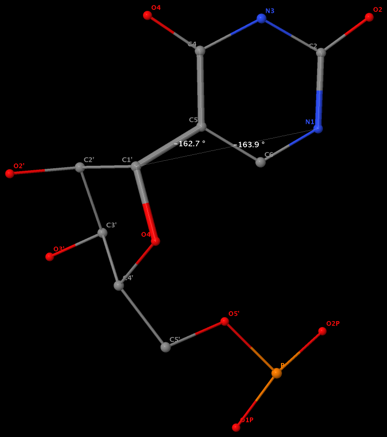
Pseudouridine (5-ribosyluracil, PSU) was the first identified modified nucleoside in RNA and is the most abundant. PSU is unique in that it has a C-glycosidic bond (C-C1′) instead of the N-glycosidic bond common to all other nucleosides, canonical or modified. It thus poses a problem as to how to calculate the χ torsion angle: should it be O4′-C1′-C5-C4, reflecting the actual glycosidic bond connection, or should the conventional definition O4′-C1′-N1-C2 still be applied literally? As a concrete example, the figure below shows the (slightly) different numerical values (–162.7° vs. –163.9°), as given by the two definitions, for PSU 6 on chain A of the PDB entry 3cgp (based on the 2009 Biochemistry article by Lin & Kielkopf titled X-ray structures of U2 snRNA-branchpoint duplexes containing conserved pseudouridines).

Needless to say, the specific definition of the χ torsion angle for PSU in RNA structures is a very subtle point, and I am not aware of any discussion on this issue in literature. In 3DNA, PSU is identified explicitly, and χ is defined by O4′-C1′-C5-C4. In NDB and a couple of other tools I am familiar with, χ for PSU is defined by O4′-C1′-N1-C2. Again using 3cgp (figure below) as an example, 3DNA gives –162.7°, whilst NDB gives –163.9°. Additionally, this distinction in N-C1′ vs. C-C1′ connection also comes into play when calculating the perpendicular distance from the 3′ phosphorus atom to the glycosidic bond, as per Richardson et al.

Except for pseudouridine, a nucleoside in DNA/RNA contains an N-glycosidic bond that connects the base to the sugar. The chi (χ) torsion angle, which characterizes the relative base/sugar orientation, is defined by O4′-C1′-N1-C2 for pyrimidines (C, T and U), and O4′-C1′-N9-C4 for purines (A and G).

Normally (as in A- and B-form DNA/RNA duplex), χ falls into the ranges of +90° to +180°; –90° to –180° (or 180° to 270°), corresponding to the anti conformation (Figure below, top). Occasionally, χ has values in the range of –90° to +90°, referring to the syn conformation (Figure below, bottom). Note that in left-handed Z-DNA with CG repeating sequence, the purine G is in syn conformation whilst the pyrimidine C is anti.

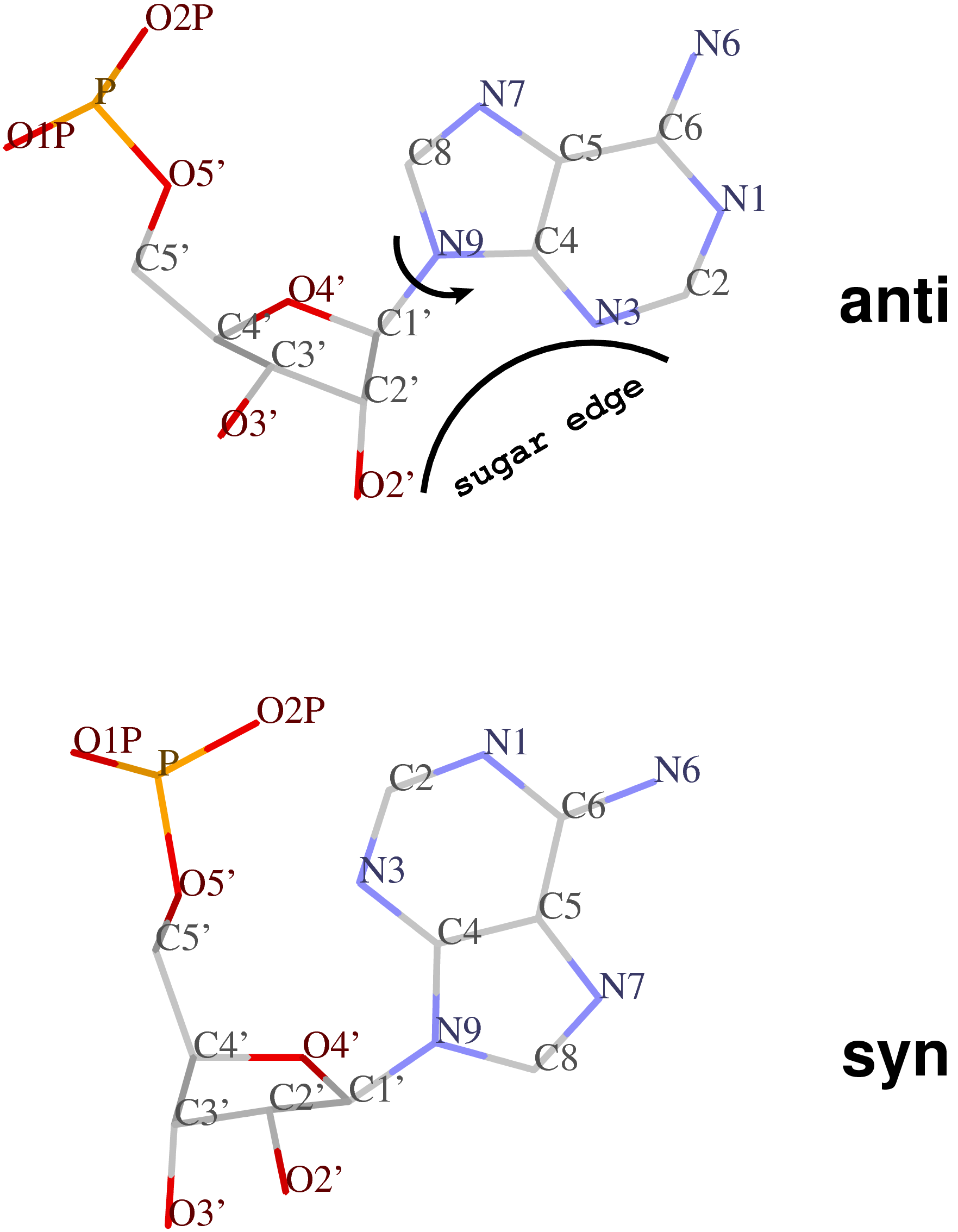
Presumably, the χ-related anti / syn conformation is a simple geometric concept. Nevertheless, the N-glycosidic bond and the corresponding χ torsion angle illustrate that the base and the sugar are two separate entities, i.e. there is an internal degree of freedom between them. In this respect, it is worth noting that the Leontis-Westhod sugar edge for base-pair classification corresponds to the anti form (as applied to RNA) only. When a base is flipped over into the syn conformation, the “sugar edge”, defined in connection with the minor (shallow) groove side of a nitrogenous bases, simply does not exist.

Base-flipping (anti / syn conformation switch) is one of the factors associated with the two possible relative orientations of the two bases in a pair, characterized explicitly in 3DNA as of type M+N or M–N since the 2003 NAR paper (Figure 2, linked below). I re-emphasized this distinction in our 2010 GpU dinucleotide platform paper (in particular, see supplementary Figure S2). Unfortunately, this subtle (but crucial, in my opinion) point has never been taken seriously (or at all) by the RNA community, even with 3DNA’s wide adoption. However, as people know 3DNA deeper/better and take RNA base-pair classification more rigorously, I have no doubt that the simplicity of this explicit distinction and the resultant full quantification of each and every possible base pair using standard geometric parameters will gradually be appreciated.

As of 3DNA v2.1, the output of the χ torsion angle is also associated with its classification in anti / syn conformation, among other new features (see for example the output for 6tna).

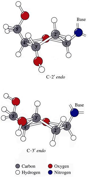
The sugar puckers in DNA/RNA structures are predominately in either C3′-endo (A-DNA or RNA) or C2′-endo (B-DNA; see Figure below, left), corresponding to the A- or B-form conformation in a duplex. In these two sugar conformations, the distance between neighboring phosphorus (P) atoms and the orientation of P relative to the sugar/bases are also dramatically different (figure below, right).

Recently, I carefully re-read some articles on RNA backbone conformation by Richardson et al., including:

• RNA backbone is rotameric (PNAS 2003)
• RNA backbone: consensus all-angle conformers and modular string nomenclature (RNA 2008)
• MolProbity: all-atom structure validation for macromolecular crystallography (Acta Crystallogr D Biol Crystallogr. 2010)
• PHENIX: a comprehensive Python-based system for macromolecular structure solution (Acta Crystallogr D Biol Crystallogr. 2010)

I became intrigued by one of their observations: i.e., the correlation between the sugar pucker and a simple distance parameter:

C3′-endo and C2′-endo sugar puckers are highly correlated to the perpendicular distance between the C1′–N1/9 glycosidic bond vector and the following phosphate: > 2.9 Å for C3′-endo and < 2.9 Å for C2′-endo. (p.16 from the MolProbity paper).

Out of curiosity and for a better understanding of this correlation, I played around with some sample cases both visually and numerically. Overall, this involves a simple geometric calculation, i.e., the shortest distance from a point to a line in three-dimensional space. Given below is the Octave/Matlab script for calculating the distances for G175 and U176 of PDB entry 1jj2 (the large ribosomal subunit of Haloarcula marismortui):

function d = get_p3_nc_dist(P3, C1, N)
    C1_N = N - C1;               # vector from C1′ to N
    nv_C1_N = C1_N / norm(C1_N); # normalized vector
    C1_P3 = P3 - C1;             # vector from C1′ to P3
    proj = dot(C1_P3, nv_C1_N);
    d = norm(C1_P3 - proj * nv_C1_N);
end

## G175
P3 = [70.104 112.366  44.586];
C1 = [73.017 109.666  45.304];
N9 = [74.445 109.380  45.288];
d1 = get_p3_nc_dist(P3, C1, N9)  # 2.2 Å -- C2′-endo

## U176
P3 = [66.871 116.402  46.804];
C1 = [68.213 112.454  49.279];
N1 = [69.678 112.480  49.438];
d2 = get_p3_nc_dist(P3, C1, N1)  # 4.6 Å -- C3′-endo

The GpU dinucleotide used in the above example forms a platform (see figure below), where the sugar of G175 adopts a C2′-endo conformation, and that of U176 C3′-endo. Indeed, the distance for G175 is 2.2 Å (< 2.9 Å); whilst the value for U176 is 4.6 Å (> 2.9 Å).

Note that the Richardson et al. articles focus on the RNA backbone, without paying attention to the base (pair) geometry. The 3DNA Zp parameter, which is the mean z-coordinate of the two P atoms in the mean reference frame of a dinucleotide step (see figure below), has been readily adapted to single-stranded RNA structures. For example, the vertical distances of the 3′ P atoms to the G175 and U176 base planes are 1.9 Å and 4.4 Å, respectively. Since base planes and the P atoms are the two most accurately located entities in a given nucleic acid structure, the nucleotide-based Zp variant is presumably more robust and discriminative than the distance from P to the glycosidic bond.

This new single-stranded based “Zp” parameter is available as of 3DNA v2.1.

RNA has three salient structural features (compared to DNA): it contains the ribose (not deoxyribose) sugar, it has the uracil (not thymine) base, and it is normally single (not double)-stranded. The O2′(G)…O2P(U) H-bond stabilized GpU dinucleotide platform may turn out to be the smallest unit with all those RNA hallmarks.

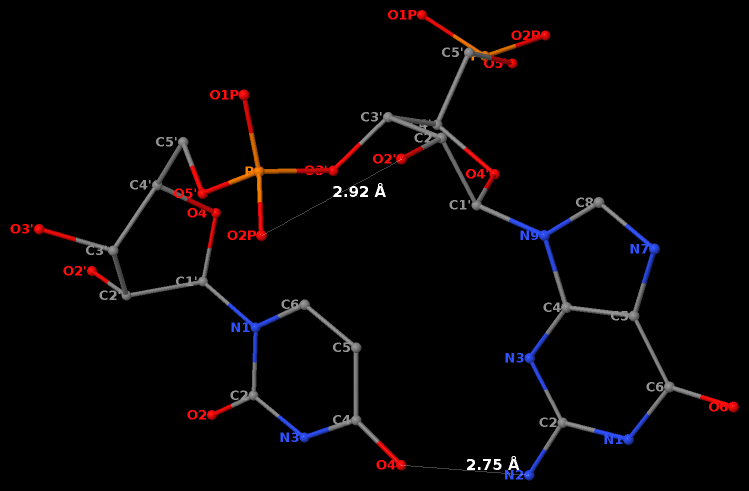
First, it must have the guanosine ribose to have the 2′-hydroxyl group form the O2′(G)…O2P(U) H-bond.

Second, the methyl group in position 5 of thymine would cause steric clash with guanosine, thus disrupting the N2(G)…O4(U) base-base H-bond to form the GpU dinucleotide platform.

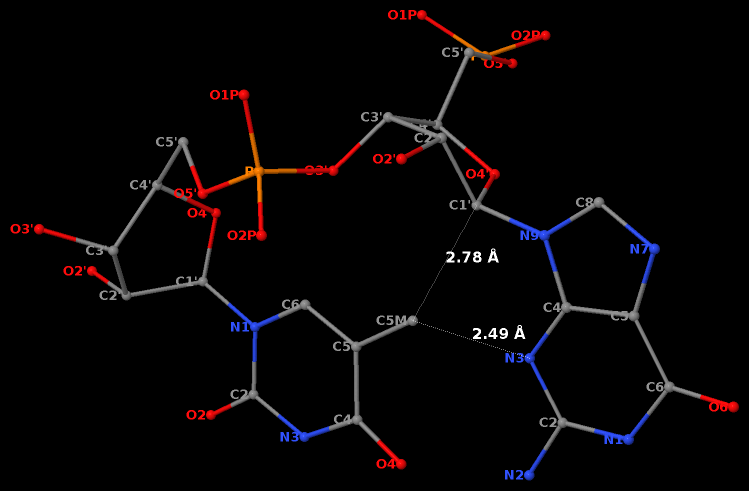
Third, a dinucleotide, by definition, is single-standed. The two H-bonds, plus the covalent linkage, makes the GpU platform extremely rigid (see Figure 1 of our 2010 NAR paper).

Moreover, the GpU platform is directional: swapping the two bases while keeping the sugar-phosphate backbone fixed does not allow for a base-base H-bond, thus no UpG dinucleotide platform.

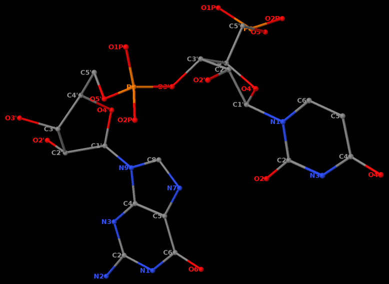
It worth noting that state-of-the-art quantum chemistry calculations have verified the importance of the O2′(G)…O2P(U) H-bond in stabilizing the GpU dinucleotide platform.

The least-squares (LS) fitting procedures presented below make use of well known mathematics. Indeed, the methods are so well known and widely used that it is somewhat difficult to locate the original references. In our previous effort to resolve the discrepancies among nucleic acid conformational analysis programs, we came across a variety of LS fitting procedures. Here we provide a detailed description, with step-by-step examples, of our implementation in 3DNA of two LS fitting algorithms based on a covariance matrix and its eigen-system. This post is the revised version of a note first made available in the “Technical Details” section of earlier 3DNA websites.

LS fitting between standard and experimental bases

Three analysis schemes — CompDNA, Curves/Curves+, and RNA — use LS procedures to fit a standard base with an embedded reference frame to an observed base structure. CompDNA and Curves/Curves+ take advantage of the conventional approach of McLachlan [“Least Squares Fitting of Two Structures.” J. Mol. Biol., 128, 74-79 (1979)], while the RNA program implements a closed-form solution of absolute orientation using unit quaternions first introduced by Horn. The two algorithms are mathematically equivalent for the most general cases, since the unit quaternion can be transformed to the rotation matrix given by McLachlan. The Horn method, however, is more straightforward and generally applicable; it can be applied even when one or both of the structures are perfectly planar, whereas the McLachlan approach fails.

Here we use the ideal adenine geometry derived from the high resolution crystal structures of model nucleosides, nucleotides, and bases. The x-, y-, and z-coordinates of the standard base, taken from the NDB, are listed below in the columns labeled sx, sy, and sz, respectively. s_(average) is the geometric center of the base.

              sx      sy      sz   
  1  N9      0.213   0.660   1.287 
  2  C4      0.250   2.016   1.509 
  3  N3      0.016   2.995   0.619 
  4  C2      0.142   4.189   1.194 
  5  N1      0.451   4.493   2.459 
  6  C6      0.681   3.485   3.329 
  7  N6      0.990   3.787   4.592 
  8  C5      0.579   2.170   2.844 
  9  N7      0.747   0.934   3.454 
 10  C8      0.520   0.074   2.491 
------------------------------------
s_(average): 0.4589  2.4803  2.3778 

We similarly describe the coordinates of one of the adenine bases (the fifth nucleotide in the sequence strand) from the high resolution (1.4 Å) self-complementary d(CGCGAATTCGCG) dodecamer duplex determined by Williams and co-workers (PDB id: 355d). The experimental xyz coordinates are listed below in the columns labeled ex, ey, and ez. The geometric center is e_(average). Note that the atomic serial numbers from the PDB (first column) have been rearranged so that the atoms are in the same order as those of the ideal base listed above.

              ex      ey      ez  
 91  N9     16.461  17.015  14.676 
100  C4     15.775  18.188  14.459
 99  N3     14.489  18.449  14.756
 98  C2     14.171  19.699  14.406
 97  N1     14.933  20.644  13.839
 95  C6     16.223  20.352  13.555
 96  N6     16.984  21.297  12.994
 94  C5     16.683  19.056  13.875
 93  N7     17.918  18.439  13.718
 92  C8     17.734  17.239  14.207
------------------------------------
e_(average):16.1371 19.0378 14.0485

We collect the two sets of xyz coordinates in the 10 × 3 matrices S and E corresponding respectively to the standard and experimental bases. We then construct the 3 × 3 covariance matrix C between S and E using the following formula:

        1             1
 C = ------- [S' E - --- S' i i' E]
      n - 1           n

   =
      0.2782    0.2139   -0.1601
     -1.4028    1.9619   -0.2744
      1.0443    0.9712   -0.6610

Here n, the number of atoms in each base, is 10, and i is an n x 1 column vector consisting of only ones. S' and i' are the transpose of matrix S and column vector i, respectively.

From the nine elements of the C matrix, we subsequently generate the 4 × 4 real symmetric matrix M using the expression:

     | c11+c22+c33     c23-c32       c31-c13        c12-c21    | 
 M = |   c23-c32     c11-c22-c33     c12+c21        c31+c13    | 
     |   c31-c13       c12+c21     -c11+c22-c33     c23+c32    | 
     |   c12-c21       c31+c13       c23+c32      -c11-c22+c33 | 

   =
      1.5792   -1.2456    1.2044    1.6167
     -1.2456   -1.0228   -1.1890    0.8842
      1.2044   -1.1890    2.3447    0.6968
      1.6167    0.8842    0.6968   -2.9011

The largest eigenvalue of matrix M is 4.0335, and its corresponding unit eigenvector is:

 [ q0   q1    q2    q3 ] = [ 0.6135   -0.2878    0.7135    0.1780 ]

The rotation matrix R is deduced from the above eigenvector as below:

     | q0q0+q1q1-q2q2-q3q3    2(q1q2-q0q3)        2(q1q3+q0q2)     | 
 R = |    2(q2q1+q0q3)     q0q0-q1q1+q2q2-q3q3    2(q2q3-q0q1)     | 
     |    2(q3q1-q0q2)        2(q3q2+q0q1)     q0q0-q1q1-q2q2+q3q3 | 

   =
     -0.0817   -0.6291    0.7730
     -0.1923    0.7710    0.6072
     -0.9779   -0.0990   -0.1839

Following coordinate transformation with matrix R, the origin of the standard base is found to be displaced from the experimental structure by:

 o = e_(average) - s_(average) R' = [15.8969 15.7701 15.1802]

The least-squares fitted coordinates (F) of the standard base atoms on the experimental structure are then given by:

 F = S R' + i o
   =
     16.4592   17.0194   14.6699
     15.7747   18.1925   14.4586
     14.4899   18.4519   14.7542
     14.1729   19.6974   14.4070
     14.9343   20.6404   13.8420
     16.2222   20.3472   13.5569
     16.9832   21.2875   12.9925
     16.6829   19.0585   13.8760
     17.9183   18.4437   13.7219
     17.7335   17.2396   14.2062

Here S is the (n x 3) matrix of original coordinates of the standard base, and as noted above, i is an n x 1 column vector consisting of only ones.

The difference matrix (D) between F and E, the (n x 3) matrix of original coordinates of the experimental base, and the root-mean-square (RMS) deviation between the two structures are found as:

 D = E - F
   =
      0.0018   -0.0044    0.0061
      0.0003   -0.0045    0.0004
     -0.0009   -0.0029    0.0018
     -0.0019    0.0016   -0.0010
     -0.0013    0.0036   -0.0030
      0.0008    0.0048   -0.0019
      0.0008    0.0095    0.0015
      0.0001   -0.0025   -0.0010
     -0.0003   -0.0047   -0.0039
      0.0005   -0.0006    0.0008

 RMS deviation = 0.0054

It should be noted that if the standard base is already defined in terms of its reference frame, as in 3DNA (e.g., $X3DNA/config/Atomic_A.pdb), the vector o and the matrix R represent the best-fitted coordinate frame of the experimental base. Moreover, the three axes of the frame given by R are guaranteed to be orthonormal. If you want to get an insight of the LS fitting algorithm and a better understanding of how 3DNA derives its base reference frame, it’d be a valuable experience to repeat the above procedure with $X3DNA/config/Atomic_A.pdb.

Note: the algorithm does not apply to a molecule vs its inversion (an improper rotation) — thanks to Boris Averkiev for reporting this subtle point (see comments below). One possible remedy is to treat this edge case separately.

Base normal

Rather than fit a standard base to experimental coordinates, the CEHS, FREEHELIX, and NUPARM analyses perform a fitting of a LS plane to a set of atoms in order to define the base and base-pair normals. The covariance matrix based on the n x 3 matrix of experimental Cartesian coordinates E is diagonalized to find the vector normal to the best plane. Specifically, C is obtained using the above formula with S substituted by E. The normal vector then lies along the eigenvector that corresponds to the smallest eigenvalue. Note that the coefficient 1/(n-1) in the formula for calculating C has no effect on the direction of the eigenvectors but scales the magnitudes of the eigenvalues.

Using the above adenine base from the high resolution dodecamer duplex as an example, the covariance matrix C is:

 C =
     1.6680   -0.5015   -0.3253
    -0.5015    2.0670   -0.5840
    -0.3253   -0.5840    0.3061

The smallest eigenvalue of C, 8.26e-5, indicates that the base is almost perfectly planar. The corresponding unit eigenvector corresponding to the base normal is:

 Base normal: 0.2737    0.3224    0.9062

Related topics:

• Automatic identification of nucleotides
• Fitting of base reference frame

As the old saying goes, a picture is worth a thousand words. To help you have a better idea of what 3DNA/DSSR is about, we’ve collected the following pictures; they serve to demonstrate selected features from 3DNA/DSSR’s versatile functionality.

Cartoon-block schematic representations generated with DSSR and PyMOL

Schematic diagram of base-pair parameters

Influence of Slide and Roll on DNA helical conformation

Roll-introduced DNA bending

Global bending of DNA associated with selective B → A conformational transformation

Canonical fiber models of A-, B-, C- and Z-DNA

3DNA-generated view of a four-way DNA–RNA junction (1egk)

3DNA-detected pentaplets in the large ribosomal subunit (1jj2)

3DNA enabled the discovery of the O2′(G)−O2P(U) H-bond which stabilizes the GpU dinucleotide platform

Nucleic-acid-containing structures generated with w3DNA

Analysis of DNA with a B-Z junction (2acj, left) and detection of hydration patterns (right)

Schematics images auto-generated via blocview

2f4u	408d	9ant

Over the years, the fiber utility program has become a handy way to generate standard B-DNA and A-DNA structures, as evident from citations to 3DNA. Nevertheless, the currently collected 55 experimental fiber models, comprehensive as they are, do not include one for canonical double-stranded (ds) RNA or single-stranded (ss) RNA structures of generic A/C/G/U sequence.

This situation is best illustrated by a recent article by Charles Brooks and Hashim Al-Hashimi and their co-workers, titled Unraveling the structural complexity in a single-stranded RNA tail: implications for efficient ligand binding in the prequeuosine riboswitch [Nucleic Acids Research, 40(3) 1345–1355 (2012)] , where they wrote:

Idealized A-form structures were constructed using Insight II (Molecular Simulations, Inc.) correcting the propeller twist angles from +15° to –15° using an in-house program, as previously described (47). The complementary strand was removed and the resulting ssRNA used in NMR data analysis. B-form helices were constructed using W3DNA (48).

As of 3DNA v2.1, however, that’s no longer the case: now the fiber utility provides direct support for generating idealized dsRNA or ssRNA structures of arbitrary A/C/G/U sequence. As always, the new functionality can be best illustrated with examples. Let’s build ssRNAs of the wild-type (5’-AUAAAAAACUAA-3’) and A29C mutated form (5’-AUAACAAACUAA-3’) used in the work cited above:

fiber -r -s -seq=AUAAAAAACUAA wt-12nt.pdb
fiber -r -s -seq=AUAACAAACUAA mt-12nt.pdb

Here the -r option is for RNA, -s for a ss structure, and -seq for the specific base sequence. The generated ssRNA structure for the wild-type sequence is named wt-12nt.pdb, and that for the mutated sequence named mt-12nt.pdb.

Note that the new RNA model is based on Struther Arnott’s work of fiber A-DNA from calf thymus (#1 in the list). The dsRNA, as its dsDNA counterpart, has a helical twist of 32.7° and a helical rise of 2.548 Å. Relevant to the above citation, here the propeller twist angle of each base pair is –10.5°, a negative value similar to that observed in high-resolution x-ray crystal structures. Furthermore, you can easily verify the three numbers with the following commands:

fiber -r -seq=AUAAAAAACUAA wt-12nt.pdb
find_pair wt-12nt.pdb stdout | analyze stdin

In summary, it is very easy to generate canonical RNA structures with the revised fiber command. Through its integrated analysis routine, 3DNA can also be used to check structural features of the resultant RNA models. Moreover, as mentioned in the opening post What can 3DNA do for RNA structures? on the forum, 3DNA has much to offer in the filed of RNA structural bioinformatics.

At the C2B2 party this afternoon, I was asked the question: “Does 3DNA work for RNA?” Well, a good question, indeed. The short answer is definitely, YES. However, a detailed explanation is needed to address the underlying intuitive assumption: 3DNA is only for DNA.

• The name 3DNA was due to Dr. Olson, after we struggled quite a while. Initially, we played with NuStar (which was actually cited once by Richard Dickerson et al.), and Carnival etc. I still remember the day when Dr. Olson asked me “How about 3DNA?” We immediately reached an agreement: that’s it — what a cute name! Another advantage (as it becomes clear later): since 3DNA starts with ‘3’, it (mostly) shows up right at the top of many on-line lists of bioinformatics tools.
• Interpreted literally, 3DNA could mean 3-DNA, i.e., the three most common types of DNA: A-, B- and Z-form. That may be one of the reasons where the misconception that 3DNA is only for 3DNA comes from. Another reason could be that structural work on DNA is what the Olson lab best known for.
• The number ‘3’ in 3DNA should also be associated with its three key components: analysis, rebuilding and visualization. In a sense, this is my favorite.
• Of course, 3DNA stands for 3D-NA, 3-Dimensional Nucleic Acids, as expressed explicitly in the titles of our two 3DNA papers (2003 NAR and 2008 NP).

The applications of 3DNA to RNA structures can be broadly categorized as follows:

• Automatically detect all existing base-pairs, Watson-Crick (A-U, G-C, wobble G-U) or non-canonical, using a set of simple geometric criteria. Furthermore, it has a unique base-pair classification system based on the six numerical structural parameters, suitable for database storage and search.
• Automatically detect all triplets or higher-order base-associations.
• Automatically detect double helical regions, regardless of backbone connection, thus ideal for finding pseudo-continuous coaxial stacking.
• The above three features are seamlessly integrated with the visualization component to allow for easy generation of publication quality images. See the 3DNA 2008 NP paper for detailed examples.

As further examples, the following two RNA publications take advantage of find_pair from 3DNA:

• R. Tyagi & D. H. Mathews (2007). Predicting Helical Coaxial Stacking in RNA Multibranch Loops. RNA, 13, 939 – 951. See the note from the authors’ webpage for clarification of mis-citation to find_pair.
• R. Capriotti & M. A. Marti-Renom (2009). SARA: a Server for Function Annotation of RNA Structures. Nucl. Acids Res., 37, W260-W265.

It is well worth noting that the base-pair detecting algorithm in RNAView is based on an earlier version of find_pair, a basic fact ignored in the RNAView publication.

In summary, 3DNA works for RNA as well as for DNA, and more.

A video overview of DSSR

DSSR (Dissecting the Spatial Structure of RNA) is an integrated software tool for the analysis/annotation, model building, and schematic visualization of 3D nucleic acid structures (see the figures below and the video overview). It is built upon the well-known, tested, and trusted 3DNA suite of programs. DSSR has been made possible by the developer’s extensive user-support experience, detail-oriented software engineering skills, and expert domain knowledge accumulated over two decades. It streamlines tasks in RNA/DNA structural bioinformatics, and outperforms its ‘competitors’ by far in terms of functionality, usability, and support.

Wide citations. DSSR has been widely cited in scientific literature, including: (i) “Selective small-molecule inhibition of an RNA structural element” (Nature, 2015; Merck Research Laboratories), (ii) “The structure of the yeast mitochondrial ribosome” (Science, 2017), (iii) “RNA force field with accuracy comparable to state-of-the-art protein force fields” (PNAS, 2018; D. E. Shaw Research), (iv) “Predicting site-binding modes of ions and water to nucleic acids using molecular solvation theory” (JACS, 2019), (v) “RIC-seq for global in situ profiling of RNA-RNA spatial interactions” (Nature, 2020), and (vi) “DNA mismatches reveal conformational penalties in protein-DNA recognition” (Nature, 2020).

Broad integrations. To make DSSR as widely accessible as possible, I have initiated collaborations with the principal developers of Jmol and PyMOL. The DSSR-Jmol and DSSR-PyMOL integrations bring unparalleled search capabilities (e.g., ‘select junctions’ for all multi-branch loops) and innovative visualization styles into 3D nucleic acid structures. DSSR has also been adopted into numerous other structural bioinformatics resources, including: (i) URS, (ii) RiboSketch, (iii) RNApdbee, (iv) forgi, (v) RNAvista, (vi) VeriNA3d, (vii) RNAMake, (viii) ElTetrado, (ix) DNAproDB, (x) LocalSTAR3D, (xi) IPANEMAP, and (xii) RNANet.

Advanced features. DSSR may be licensed from Columbia University. DSSR Pro is the commercial version. It has more functionalities than DSSR basic (the free academic version), including: (i) homology modeling via in silico base mutations, a feature employed by Merck scientists, (ii) easy generation of regular helical models, including circular or super-helical DNA (see figures below), (iii) creation of customized structures with user-specified base sequences and rigid-body parameters, (iv) efficient processing of molecular dynamics (MD) trajectories, (v) detailed characterization of DNA-protein or RNA-protein spatial interactions, and (vi) template-based modeling of DNA-protein complexes (see figures below). DSSR Pro supersedes 3DNA. It integrates the disparate analysis and modeling programs of 3DNA under one umbrella, and offers new advanced features, through a convenient interface. For example, with the mutate module of DSSR Pro, one can automatically perform the following tasks: (i) mutate all bases to Us, (ii) mutate bases in hairpin loops to Gs, and (iii) mutate G–C Watson-Crick pairs to C–G, and A–U to U–A. Moreover, DSSR Pro includes an in-depth user manual and one-year technical support from the developer.

Quality control. DSSR is a solid software product that excels in RNA structural bioinformatics. It is written in strict ANSI C, as a single command-line program. It is self-contained, with zero runtime dependencies on third-party libraries. The binary executables for macOS, Linux, and Windows are just ~2MB. DSSR has been extensively tested using all nucleic-acid-containing structures in the PDB. It is also routinely checked with Valgrind to avoid memory leaks. DSSR requires no set up or configuration: it simply works.

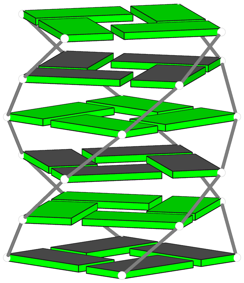
Theoretical models of G-quadruplexes, created using DSSR Pro.

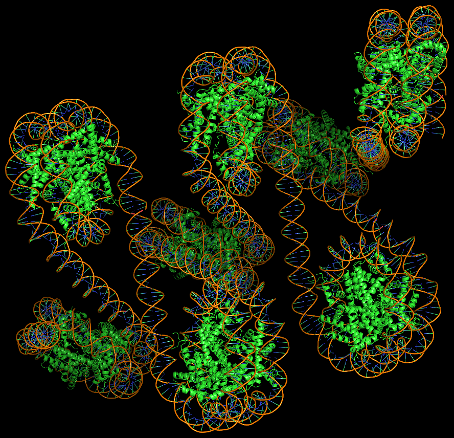
Template-based modeling of DNA-protein complexes using DSSR Pro.
Here are two chromatin-like models using PDB entry 4xzq as the template.

Circular DNA duplexes modeled using DSSR Pro.

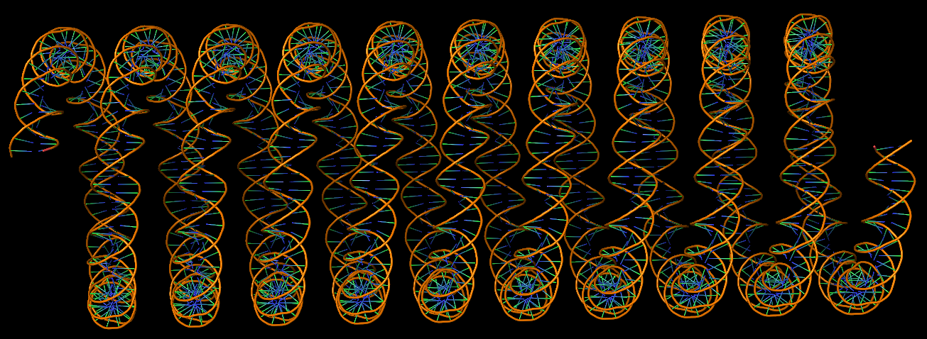
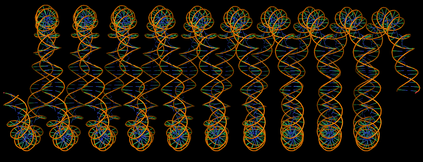
DNA super helices modeled using DSSR Pro.

Innovative cartoon-block schematics enabled by the DSSR-PyMOL integration for six representative PDB entries. Watson-Crick pairs are shown as long blocks with minor-groove edges in black (A, B), G-tetrads represented as square blocks and the metal ion as sphere ©, the ligand rendered as balls-and-sticks (D), and proteins depicted as purple cartoons (E, F). Color code for base blocks: A, red; C, yellow; G, green; T, blue; U, cyan; G-tetrad, green; WC-pairs, per base in the leading strand. Visit http://skmatic.x3dna.org.
Recommended in Faculty Opinions: “simple and effective”, “Good for Teaching”.
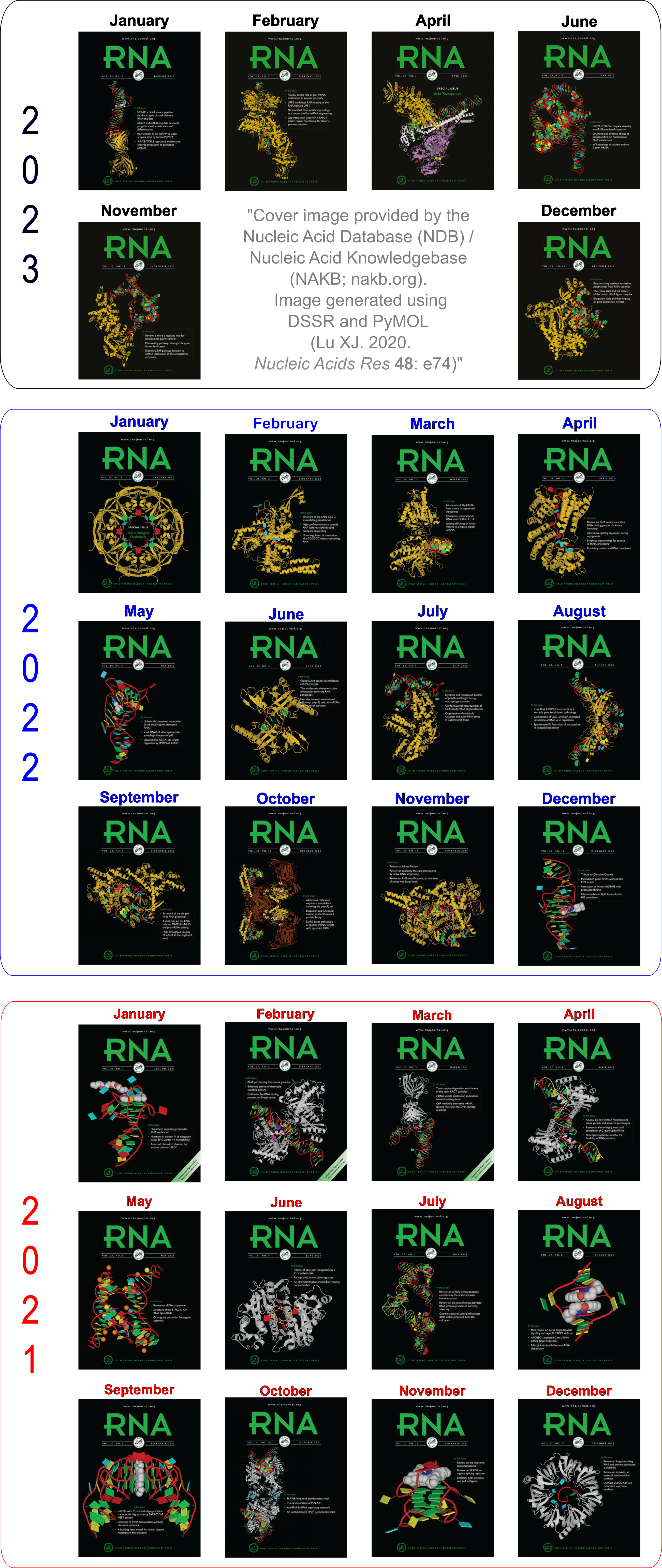
Employed by the NDB to create cover images of the RNA Journal.

References

- Geng A, Roy R, Ganser L, Li L, Al-Hashimi HM. Revealing hidden protonated conformational states in RNA dynamic ensembles. Nucleic Acids Research. 2025;53:gkaf1366. https://doi.org/10.1093/nar/gkaf1366.
- Gordan R, Wasserman H, Chi B, Bohm K, Duan M, Sahay H, et al. High-throughput characterization of transcription factors that modulate UV damage formation and repair at single-nucleotide resolution. 2025. https://doi.org/10.21203/rs.3.rs-8197218/v1.
- Kubaney A, Favor A, McHugh L, Mitra R, Pecoraro R, Dauparas J, et al. RNA sequence design and protein–DNA specificity prediction with NA-MPNN. 2025. https://doi.org/10.1101/2025.10.03.679414.
- Glasscock CJ, Pecoraro RJ, McHugh R, Doyle LA, Chen W, Boivin O, et al. Computational design of sequence-specific DNA-binding proteins. Nat Struct Mol Biol. 2025;32:2252–61. https://doi.org/10.1038/s41594-025-01669-4.
- Si Y, Xu Y, Chen L. End-to-end single-stranded DNA sequence design with all-atom structure reconstruction. 2025. https://doi.org/10.64898/2025.12.05.692525.